Solar Availability in Cities

Introduction

Dense urban habitats with residential or commercial towers make for a very complex environment where self-shading and overshadowing by adjacent buildings can significantly impact solar energy potential and daylight availability. This in turn leads to reductions in solar heat gains through windows and less than adequate access to daylight. These types of environments can vary significantly from site to site, depending on their latitude, separation distances between buildings and their height, among other things. Therefore, since such information can be site specific, it becomes difficult to use a set of generic rules as a means of providing guidelines on solar and daylighting design. The use of simulation tools becomes a necessity in this case in order to predict the dynamic effects of surface overshadowing at an urban scale.

In addition, building regulations are becoming increasingly more stringent as regards to the energy performance of buildings. This is especially true in Europe, where EU Directives are driving fundamental changes in the way buildings are designed. Solar access and right-to-light regulations can place specific limitations to the geometry of a scheme. It therefore becomes necessary to have a means of assessing the solar and daylight potential of a site, even before a building is designed. The methods proposed provide that means, by allowing an assessment of solar and daylight potential for any complex urban site.

In this paper we propose a new approach, where the information a designer needs is available in a visually meaningful way. The information presented, should allow the designer to make an assessment of where the desirable boundaries lie. For example, assess in a simple manner whether a particular site has the potential to receive the desired solar radiation, or what the height, width and length limits would be for a building to receive a certain amount of radiation, without compromising the radiation collected from nearby buildings.

This approach to calculating and visualising solar availability is a design approach, since its main purpose it to inform our design. To achieve this, two methods are presented for calculating and visualising the desired metrics. The first part of the paper deals with mapping solar radiation and other metrics on buildings surfaces and the second part, deals with calculating the full spatial variation in solar availability over the entire un-built volume of a site using a grid.

In both methods proposed, there are a number of parameters that can be calculated. The way the methods are developed allows for the storage and easy access and display of a number of those metrics within the same model. First of all solar availability, which can be characterised by the amount of total solar radiation received over a whole year. This is essentially the total global radiation, which can be subdivided into its components of direct and diffuse radiation. Part of the collected solar radiation is useful for photosynthesis in plants, this is called Photosyntherically Active Radiation (PAR) and is a parameter of substantial significance in cities, since plant and grass growth can significantly improve urban environments. Another useful parameter is daylight availability, which can be characterised at an urban scale by daylight factors, daylight levels, BRE vertical sky component, daylight and shaded hours, among others. The methods proposed, allow for all these values to be calculated, visualised and stored within the same model.

Mapping Over Surfaces

A significant amount of work has been undertaken in recent years on calculating and mapping the effects of overshadowing on solar radiation in dense urban environments. Notable examples include a method for calculating solar radiation in all types of surfaces, either in open urban environments or inside buildings (Sanchez et al., 2005); an irradiance calculation method for horizontal or tilted shaded surfaces (Quaschning and Hanitsch, 1998); a simulation based approach where RADIANCE (Ward and Shakespeare, 1998) and weather data are used to calculate irradiance over any period of time. The results can then be visualised on static images produced by the software, where irradiance is mapped on building surfaces. This can be extended to a larger scale and integrated to a GIS system (Mardaljevic and Rylatt, 2003). A limitation of this method, is that it requires the generation of a number of images in order to visualise the irradiance distribution over all building surfaces, making the simulation process more timely. In addition, every image can hold one piece of information, which necessitates the use of multiple images of the same view, in order to compare different cases or metrics. When assessing the potential impact on solar availability of alternative design schemes, these methods can significantly delay the process, while not helping designers much in understanding the limitations of a particular site and thus allowing them to provide more design solutions.

New Approach

The method proposed here deals with this issue and allows a 3D interactive environment for designers to explore, with the flexibility of having a number of values stored for each surface so that easy comparisons can be performed within the same model.

In order to develop both proposed methods, the environmental design analysis software ECOTECT (Marsh, 1996) was used. To map solar radiation or any other metric on surfaces, every surface of each building was divided into smaller segments. For a each segment, a shading mask was calculated to capture the surrounding geometry and their overshadowing effects on that surface. Then, the cumulative incident solar radiation collected throughout the year was calculated based on a weather file for that location. The solar radiation collected, as well as other metrics can be calculated for any specific period of the year. There is no limitation to how small each surface can be, the smaller it is, the more accurate the results will be. The flexibility of the system, allows for a number of different metrics to be stored for the same surface. For example, each surface can contain the values of global, direct and diffuse radiation for a whole year, as well as daylight levels among others. This allows for easy comparison between different metrics as well as data manipulation to perform simple statistical analyses, all within the same model.

Applications

The usefulness of the information provided can range from basic design guidelines to designers on how to best utilise the site’s solar boundary conditions, to providing rough estimates to local authorities about solar access rights.

Mapping solar radiation and other metrics on surfaces can tell us a lot about the complex overshadowing effects present in cities. This, can guide us into positioning PV panels in the most effective location. In addition, it can help us determine whether we need the whole skin of a building to be uniform. Work by one of the authors (Marsh, 2004), suggests that depending on the solar radiation collected, we can alter the properties of the fabric of a building to respond to the changing levels of radiation collected throughout a façade.

Example Case Studies

Figure 1 shows an example of a highly built up area, containing high-rise towers, where the total yearly solar radiation collected has been mapped over the building surfaces. The lighter tones indicate higher values and darker tones smaller values. It is obvious that the complex overshadowing effects present on this site, produce a variation in solar availability in all buildings which depends on height, exposure direction and location within the site. The flexibility of the software used allowed us to interactively pan, zoom in and rotate the model to get a better view of the area we were interested in and thus visually capture the variation in solar radiation collected.

In figure 2 we can compare the variation in Global yearly incident radiation over North and West facing surfaces. Similarly, we can compare the variation in Direct, or Diffuse radiation, or other metrics by simply choosing to display the relevant value. This allows us for example, to quickly assess the contribution Direct or Diffuse radiation in each surface. Figure 2, clearly shows that the contribution of diffuse radiation in most buildings is much greater than the direct on most of the displayed surfaces.

Mapping over surfaces also allows us to map other metrics then solar radiation. In the example of figure 3, we have mapped the shading potential in terms of yearly shaded hours for each surface of the adjacent buildings, for two different design schemes. To get an accurate comparison between the two schemes, we have subtracted the values obtained from one scheme from the other and all this within the same model. This way, the emerging image could point out which scheme performed better overall and highlight areas, where one design performed better than the other.

Another way of obtaining useful information, is to calculate the required metrics over specific surfaces, rather than the whole building. That way, significant time savings can be achieved and a quick assessment can be made before a full-run for all the surfaces is performed. The flexibility of the software used, allowed the use of other dedicated simulation software, such as RADIANCE, to perform specific calculations. In the case presented in figure 4, surfaces on five levels were selected and with the use of RADIANCE, vertical daylight factors were calculated and then imported back into the model. The distance between the calculated surfaces did not allow for the variations to be easily visually captured, as a result the values were represented in vectors.

Limitations

Mapping solar radiation or other metrics over surfaces allows us to visualise their effect in great detail in urban environments. When assessing an existing or a proposed scheme this is very useful, but if we are at a pre-design stage and want to inform our design, mapping over surfaces does not help much. It requires us to interpolate the calculated data and make a judgement on the direction our design should progress towards. For example, on an un-built site we can assess what the current collection of solar radiation is over nearby building surfaces as well as the ground surface of the site. Although this information is useful, it does not tell us much about how our design should progress, in order for it not to have an adverse effect on nearby buildings, be compliant with regulations as well as our own requirements. The only way we can assess the impact of a scheme is to design it, test what effect it has and depending on the outcome either finalise the design, or redesign it and test it again until it is compliant. This leads us to a trial and error approach, as summarised by figure 5. If we are at a pre-design stage though where no design has been finalised yet and we want to inform our design, rather than assess a proposal, modify it and re-assess it, then mapping over surfaces becomes a timely and less informative approach.

Case for an Alternative Approach

What is needed is a way to visually represent the solar potential that a particular urban area has. A method, where the impact surrounding buildings have on solar radiation can be visualised for an un-built site over its full 3D extends. That way an assessment can be made on the solar availability of any site without a design been realised yet. Although solar radiation is one of the key physical quantities in an urban environment, other metrics should similarly be represented like daylight factors and photosynthetically active radiation, among others, which can complement our understanding and inform our design. The presentation of this information in a simple and easily understandable manner would be central in realising such a method.

We therefore propose a method, where solar availability as well as other metrics are mapped over the 3D space in between buildings. To achieve this, a grid point system is used with the required metrics being calculated for each point in the grid. The flexibility of the grid, allows us to represent in 3D the iso-levels/boundaries at which a particular value is reached. We can therefore know for example, where the boundaries lie in terms of X, Y and Z coordinates for a value of 300 Wh/m² to be reached.

Spatial Solar Availability

In addition to calculating the distribution of solar radiation over a series of existing building surfaces, it is possible to calculate the full spatial variation in solar availability over the entire volume of a site. This is especially important at pre-design stage, where only the effects of buildings surrounding the site need be considered. This allows designers to respond to 3-dimensional patterns of solar availability in order to make best use of what is becoming a limited resource in increasingly built-up urban areas.

This process involves extending a 3-dimensional grid of points over the area of interest. Obviously the extents of the grid and the number of points in each cardinal dimension are user-definable. A solar availability calculation is then carried out for each point and stored within the grid.

Incidence on Surfaces and Points

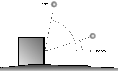
When calculating solar incidence on a surface, the cosine law is applied to account for changing angles of incidence for both the direct sun and for the distribution of diffuse radiation over the sky dome. This means that, for a vertical surface, radiation from the zenith of the sky contributes much less than radiation from the horizon directly in front of the surface. It also means that surfaces facing east, west or away from the equator are exposed to proportionally less solar radiation over time that those facing towards the equator.

This is not the case for points within the analysis grid as they have no discernable ‘direction’ or orientation. Whilst it is possible to assign artificial surface vectors to each grid point, at pre-design stage there is usually no building design from which to draw this information. If a vector is assigned, then each point is considered to be a ‘small’ surface with a normal pointing in the direction of the vector and incidence angles fully considered. If no vector is assigned, then each point acts as a spherical sensor, equally sensitive to solar radiation from all directions.

Spatial Visualisation Techniques

Once calculations are complete over the full 3D grid of points, it is possible to both quantify and visualise the results. Visualising spatial information in a way that is useful to the designer is notoriously difficult. In many cases simple slices through the 3D grid, both horizontally and vertically, can reveal useful information and identify the nature of variations ins specific parts of the modeled site. Figure 7 below shows some examples of 2D slices taken through the 3D analysis grid.

It is also possible to display the full 3D grid data volumetrically, applying variable transparency to each grid cell based on its relationship to a set threshold. In its simplest form, this means only showing those grid cells whose average values are below a user-definable threshold. The image to the left in Figure 8 below shows an example of this visualization technique.

An alternate method is to apply continuous variation in the level of transparency of each cell based on a minimum and maximum value range. Any cell with a value at or above the maximum is fully transparent whilst any cell at or below the minimum is fully opaque. Between these two values the transparency is linearly interpolated. The image on the right in Figure 8 shows an example of continuous transparency effects.

Interactive View Manipulation

Whilst not shown here, this technique is particularly effective when combined with colour variation over the same scale and the ability to interactively rotate the model. One of the benefits of the implementation described in this work is that it allows the design team to interact with the model visualization. Using the OpenGL graphics platform, all but the largest and most complex grids can be panned and rotated in close to real-time. This animation and movement of the 3D model greatly assists the viewer’s perception of depth and form within the semi-transparent mass of grid cells.

Thresholds Analysis

Another visualisation technique that can be applied to solar availability involves drawing 3D isopleths through the analysis grid at a user-defined threshold value. This establishes a virtual surface over the site, above which values of solar radiation exceed the threshold. This can be a useful early design tool in that it clearly defines how high a new building form needs to be in order to gain the desired solar exposure. The images in figure 9 show examples of these isopleths for both global and diffuse solar radiation values.

The informational and contextual benefit of 3D isopleth images is based on the ability to interactively change the threshold value to see the rates of change in different parts of the site. For example, figure 10 shows the same site analysis grid with isopleths at three different threshold values - 300, 250 and 200 Wh/m².

Isolating Individual Building Effects

This technique can also be applied to individual buildings within a site in order to quantify their overshadowing effects. This way it is possible to visualise the potential effect of a proposed building on those that surround it. Figure 11 below illustrates just such a situation, where the potential global, direct and diffuse impact of a large office tower can be considered very early in the design process.

Practical Applications

3D volumetric mapping can also help us determine the most effective location for positioning plants, trees and grass. By predicting the availability of photosynthetically active radiation, we can determine where grass growth will be viable. In addition, if we are to expand the 3D-volumetric mapping over a whole city, we can predict and visually indicate regions of the city that receive more or less radiation than a specified value.

Conclusions

In this paper we have presented two ways of visualising and calculating solar availability in cities. The first method dealt with mapping solar radiation as well as other metrics on building surfaces. This approach was found to be more suitable in assessing existing schemes, determining the most effective location for renewables and performing comparisons on the effect different schemes might have on surrounding building. This approach was not found to be suitable at a pre-design stage, where no design scheme has been realised yet. The second method, dealt with calculating the spatial variation of solar radiation over the entire un-built volume of a site. This proposed method was found to be more suitable at a pre-design stage, to determine the 3D spatial extends of desired, or acceptable solar radiation limits. Both methods can complement each other, with the second method being used at an earlier pre-design stage where the volume of a scheme needs to be determined, so that it complies with legislation. Then, the first method being used to compare the impact of different possible acceptable designs on nearby buildings. Both methods are capable of handling complex 3D geometries, while retaining their accuracy.

References

- Mardaljevic, J., Rylatt, M. 2003. Irradiation mapping of complex urban environments: an image-based approach. Energy and Buildings 35, 27-35.
- Marsh, A.J. 1996. Performance Modelling and Conceptual Design. Proceeding of the international IBPSA conference. The University of New South Wales, Sydney, Australia.
- Marsh, A.J., 2004. Calculating variations in the Distribution of InsolationOver Building Surfaces. Proceedings of the international conference on Building Envelope Systems and Technologies. Sydney, Australia, 2004.
- Quaschning, V., Hanitsch, R. 1998. Irradiance calculations on shaded surfaces. Solar Energy 62 (5), 369-375.
- Sanchez, F.J., Cebolla, R.O., Felix, J.L.M., Dominguez, S.A., 2005. Solar radiation calculation methodology for building exterior surfaces. Solar Energy 79, 513-522.
- Ward, G.J., Shakespeare, R., 1998. Rendering with Radiance: The Art and Science of Lighting Visualization, Morgan Kaufmann, San Francisco.